Terrascope logoProba-V MEP logo
The FAQ applies to Terrascope and Proba-V MEP. Please note that the FAQ is in English only.

Frequently asked questions

Developer Guide

How to write Python scripts?

Here are some important tips when working with Python.

Recommended versions

We preinstalled and configured Python 3.6 on all user VMs and on the processing cluster. This is currently the default version. Python 3.5 support is also available on the VMs and the cluster.

To switch to the Python 3.5 environment, you should run:

scl enable rh-python35 bash

Once inside this environment, all commands will default to using Python 3.5.

To use the Python 3.6 environment, you should run it using the Python3.6 binary in your VM


Installing packages

Even though we already provide a number of widely used Python packages by default, you probably need to install some new ones at some point. We recommend doing this using the pip package manager. For example:

pip install --user owslib

Installs the owslib library. The '--user' argument is required to avoid needing root permissions and to ensure that the correct Python version is used. Do not use the yum package manager to install packages!

More advanced options are explained here: https://proba-v-mep.esa.int/documentation/manuals/python-package-management

On the processing cluster

To run your code on the cluster, you need to make sure that all dependencies are also available. However, it is not possible to install specific packages on the cluster, but feel free to request the installation of a specific package.

If more freedom is needed, it is also possible to submit your dependencies together with your application code. This is simplified if you are already using a Python virtual environment for your development.

A non-exhaustive list of currently installed standard Python packages is given below.

affine, catalogclient, Cython, dask, dataclient, docker, Fiona, GDAL, geojson, geopandas, h5py, matplotlib, netCDF4, numpy, pandas, pyproj, rasterio, scipy, seaborn, sentinelhub, sentinelsat, tensorflow, xarray.

The complete list of standard installed packages can be obtained using the command 'pip3.6 freeze'.

Sample project

Two sample Python/Spark projects are available on Bitbucket; they show how to use Spark (https://spark.apache.org/) for distributed processing on the Terrascope Platform.

The basic code sample implements an (intentionally) very simple computation: for each PROBA-V tile in a given bounding box and time range, a histogram is computed. The results are then summed and printed. The computation of the histograms runs in parallel.

The project's README file includes additional information on how to run it and inspect its output.

The advanced code sample implements a more complex computation: it will calculate the mean of a time series of PROBA-V tiles and output it as a new set of tiles. The tiles are being split up into sub-tiles for increased parallelism. A mean is just an example an operation that can be applied to a time series.

Application specific files

Auxiliary data

When your script depends on specific files, there are a few options:

Use the --files and --archives options of the spark-submit command to put local files in the working directory of your program, as explained here.
Put the files on a network drive, as explained here.
Put the files on the HDFS shared filesystem, where they can be read directly from Spark, or can be placed into your working directory using --files or --archives.

The second option is mostly recommended for larger files. The other options are quite convenient for distributing various smaller files. Spark has a caching mechanism in place to avoid unneeded file transfers across multiple similar runs.

Compiled binaries

When using compiled code, such as C++, code compiled on your VM will also work on the cluster. Hence you can safely use the compilation instructions of your tool to compile a binary, and then distribute it in a similar way as any other type of auxiliary data. In your script, you may need to configure environment variables such as PATH and LD_LIBRARY_PATH to ensure that your binaries can be found and are being used.


How to get data to the Terrascope platform?

Introduction

Each Terrascope VM user has it's own Public and Private folder, available under /data/users/Public/<username> and /data/users/Private/<username>. There is also a link to those folders in your Terrascope VM home folder (/home/<username>).

The Public folder can be used to share data with other Terrascope users as all Terrascope users can read the data, but it is only writeable by you. The Private folder is only readable and writeable by you. These folders are accessible from the Terrascope user VMs, the Hadoop cluster, and the notebooks.

Data can be uploaded by SFTP, as described below.

Importing small amounts of data on the VM

To import data to the user VM with sizes of a couple of Gigabytes or less, the easiest way would be to use an SFTP client.
For Windows, WinSCP is a good choice.
Download WinSCP (or any other SFTP client) and start it up.

Connect WinSCP to our SFTP server: filetransfer.terrascope.be.
The login credentials are the same as your VM, meaning your Terrascope username and password.

In the SFTP server you will find the folders that are shared over the entire Terrascope cluster. Your Private folder will be under /data/users/Private/<username> and you Public folder will be under /data/users/Public/<username>.

How to launch interactive applications: QGis?

Instead of launching applications in a virtual desktop environment, it is often more convenient if you can immediately start an application. The X2Go program explained on the previous page supports this. Just follow the same steps for setting up a connection as described there (MAKE ANCHOR ), but now select 'Published applications' under 'Session type' when you set up your session.

Now click on the circle icon after launching this session as shown here:

Published Apps1

This show a window where you can select an application, clicking start will launch QGis directly, as if it were running on your machine. However, you do have access to the Terrascope EO data archive!

lauching qgis


How to use Spark for distributed processing?

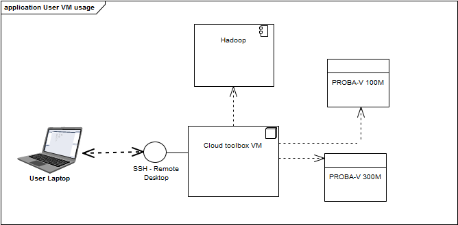
To speed up processing, it is often desirable to distribute the work over a number of machines. The easiest way to do this is to use the Apache Spark processing framework. The fastest way to get started, is to read the Spark documentation: https://spark.apache.org/docs/2.3.3/quick-start.html.

The Spark version installed on our cluster is 2.3.3 so it is recommended that you stick with this version. It is however not impossible to use a newer version if really needed. Spark is also installed on your virtual machine, so you can run 'spark-submit' from the command line after setting the following 2 environment variables:

export SPARK_MAJOR_VERSION=2
export SPARK_HOME=/usr/hdp/current/spark2-client

To run jobs on the Hadoop cluster, the 'cluster' deploy-mode has to be used, and you need to authenticate with Kerberos. For the authentication, just run 'kinit' on the command line. You will be asked to provide your password. Two other useful commands are 'klist' to show whether you have been authenticated, and 'kdestroy' to clear all authentication information. After some time, your login will expire, so you'll need to run 'kinit' again.

Python Spark example is available which should help you to get started.

Resource management

Spark jobs are being run on a shared processing cluster. The cluster will divide available resources among all running jobs, based on certain parameters.

Memory

To allocate memory to your executors, there are two relevant settings:

The amount of memory available for the Spark 'Java' process: --executor-memory 1G

The amount of memory for your Python or R script: --conf spark.yarn.executor.memoryOverhead=2048

If you need more detailed tuning of the memory managment inside the Java process, you can use: --conf spark.memory.fraction=0.05

Number of parallel jobs

The number of tasks that are processed in parallel can be determined dynamically by spark. Therefore you should use these parameters:

--conf spark.shuffle.service.enabled=true --conf spark.dynamicAllocation.enabled=true

Optionally, you can set upper or lower bounds:
--conf spark.dynamicAllocation.maxExecutors=30 --conf spark.dynamicAllocation.minExecutors=10

If you want a fixed number of executors, use:
--num-executors 10

We don't recommend this, as it reduces the ability of the cluster manager to optimally allocate resources.

Dependencies

A lot of commonly used Python dependencies are preinstalled on the cluster, but in some cases, you want to provide your own.

The first thing you need to do this, is to get a package containing your dependency. PySpark supports zip, egg, or whl packages. The easiest way to get such a package is by using pip:

pip download Flask==1.0.2

This will download the package, and all of its dependencies. Pip will prefer to download a wheel if one is available, but may also return a ".tar.gz" file, which you will need to repackage as zip or wheel.

To repackage a tar.gz as wheel:

tar xzvf package.tar.gz

cd package

python setup.py bdist_wheel

Note that a wheel may contain files that are dependent on the version of Python that you are using, so make sure you use the right (2.7 or 3.5) Python to perform this command.

Once the wheel is available, you can include it in your spark-submit command:

--py-files mypackage.whl

Notifications

If you want to receive a notification (e.g. an email) when the job reaches a final state (succeeded or failed), you can add a SparkListener on the SparkContext for Java or Scala jobs:

SparkContext sc = ... sc.addSparkListener( new SparkListener() { ... @Override public void onApplicationEnd(SparkListenerApplicationEnd applicationEnd) {   // send email   }   ... });

You can also implement a SparkListener and specify the classname when submitting the Spark job:

spark-submit --conf spark.extraListeners=path.to.MySparkListener ...

In PySpark, this is a bit more complicated as you will need to use Py4J:

class PythonSparkListener(object): def onApplicationEnd(self, applicationEnd): // send email   # also implement other onXXX methods class Java: implements = ["org.apache.spark.scheduler.SparkListener"]
sc = SparkContext() sc._gateway.start_callback_server() listener = PythonSparkListener() sc._jsc.sc().addSparkListener(listener) try: # your Spark logic goes here ... finally: sc._gateway.shutdown_callback_server() sc.stop()

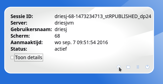
In a future release of the JobControl dashboard, we will add the possibility to send an email automatically when the job reaches a final state.


What if I don't see a background map in the Terrascope viewer?

We have noticed that sometimes the background map does not appear in the viewer. The cause of this is that the user has tracking blocker software installed. Please read this document to find out how to resolve this issue

Notebooks

What is a Notebook?

A notebook is a web application that allows you to create and share documents that contain live code, equations, visualizations and narrative text.
It is based on the Open Source Jupyter notebooks application, and tailored to the needs of remote sensing users. Each notebook has direct access to the Terrascope, PROBA-V, SPOT-VGT and Copernicus Global Land datasets.

How to work with Notebooks?

Notebooks are only enabled for users on specific demand. If you want notebook access, use the 'Request notebook access' form.

On https://notebooks.terrascope.be, you can login to the notebooks application with your Terrascope username and password, which is the same account as used on www.vito-eodata.be or PROBA-V MEP.

Notebook samples

By default, some sample notebooks are provided under folder Private/notebook-samples. You may want to run git pull inside this directory to get the latest version.

The samples are subdivided in two sections:

  • datasets: notebooks using either Sentinel or PROBA-V data
  • tools: notebooks using tools provided by the Terrascope platform (e.g. SNAP, R, catalogclient, etc ...)

Sharing notebooks

See here.

Installing additional packages

See here.

Leaflet support in older (<3.6) Python versions?

In the jupyterlab interface leaflet support is broken for Python35. However, it can still be used when you switch to the Jupyter classic interface (via Help > Launch classic notebook). Another option is migrating to Python36 where leaflet works in both the lab and classic interfaces.

Sentinel 1

What are the processing steps for the Sentinel-1 GRD sigma0 product?

A full description can be found in the TERRASCOPE SENTINEL-1 ALGORITHM THEORETICAL BASE DOCUMENT (ATBD).

Which region of interest is available now for the Sentinel-1 products?

What is the file format of the Sentinel-1 products?

  • SENTINEL data products are distributed using a SENTINEL-specific variation of the Standard Archive Format for Europe (SAFE) format specification. The SAFE format has been designed to act as a common format for archiving and conveying data within ESA Earth Observation archiving facilities. SAFE was recommended for the harmonisation of the GMES missions by the GMES Product Harmonisation Study.

The SENTINEL-SAFE format wraps a folder containing image data in a binary data format and product metadata in XML. This flexibility allows the format to be scalable enough to represent all levels of SENTINEL products.

A SENTINEL product refers to a directory folder that contains a collection of information. It includes:

  • a 'manifest.safe' file which holds the general product information in XML
  • subfolders for measurement datasets containing image data in various binary formats
  • a preview folder containing 'quicklooks' in PNG format, Google Earth overlays in KML format and HTML preview files
  • an annotation folder containing the product metadata in XML as well as calibration data
  • a support folder containing the XML schemes describing the product XML.

(Referentie: https://sentinel.esa.int/web/sentinel/user-guides/sentinel-1-sar/data-formats/safe-specification)

Sentinel 2

What is the file format of the Sentinel-2 derived biophysical products?

All Sentinel-2 image files are delivered in GeoTIFF format. The accompanied metadata file is in XML format following the INSPIRE metadata standard (ISO19115).

VITO offers 6 Sentinel-2 vegetation indices or biophysical parameters: fAPAR, fCover, LAI, CCC, CWC and NDVI. All products of these vegetation indices contain 4 files. Three datafiles (the respective biophysical parameter, a quicklook image file, and the Scene Classification), as well as the earlier mentioned XML metadata file. The data are available at both 10 m and 20 m resolution.

The table below lists the technical information of the Sentinel-2 derived products providing information on how to calculate the Physical Values (PV) from the Digital Numbers (DN) available in the files. The PV can be calculated using the following formula:

Physical Value = Scaling * Digital Number + offset.

Table: Sentinel-2 derived vegetation products Physical Value and Digital Number data range, scaling, and offsets.


FAPAR

FCOVER

LAI

NDVI

Physical min

0.0

0.0

0.0

-0.08

Physical max

1.0

1.0

10.0

0.92

Digital number min

0

0

0

0

Digital number max

200

200

250

250

Scaling

1/200

1/200

10/250

1/250

Offset

0.0

0.0

0.0

-0.08

No data

255

255

255

255

Data type

Byte

Byte

Byte

Byte

Saturation min*

/

/

/

-1.0

Saturation max**

/

/

/

1.0

*Values between saturation min and physical min will be set to physical min before quantization is applied.

** Values between saturation max and physical max will be set to physical max before quantization is applied.

More information on the biophysical parameters' retrieval methodologies can be found in the TERRASCOPE SENTINEL-2  ALGORITHM THEORETICAL BASE DOCUMENT (ATBD) S2 – NDVI & BIOPAR – V200

.

What does the scene classification map look like?

All products are delivered together with the scene classification map, which gives an indication on the pixel quality of the delivered product. The different values and their meaning are given in the table below.

Table: Pixel quality classification map

Label

Classification

0

NO_DATA

1

SATURATED_OR_DEFECTIVE

2

DARK_AREA_PIXELS

3

CLOUD_SHADOWS

4

VEGETATION

5

BARE_SOIL

6

WATER

7

CLOUD_LOW_PROBABILITY

8

CLOUD_MEDIUM_PROBABILITY

9

CLOUD_HIGH_PROBABILITY

10

THIN_CIRRUS

11

SNOW


How do we derive NDVI and biophysical parameters?

“Terrascope offers ready-to-use information products derived from Sentinel-2 data. These include

  • NDVI – Normalised Vegetation Index
  • fAPAR – fraction of Absorbed Photosynthetically Active Radiation
  • fCOVER – fraction of Vegetation Cover
  • LAI – Leaf Area Index
  • CCC – Canopy Chlorophyll Content
  • CWC – Canopy Water Content

To learn more about how these products are produced, please read the TERRASCOPE SENTINEL-2  ALGORITHM THEORETICAL BASE DOCUMENT (ATBD) S2 – NDVI & BIOPAR – V200

What is the new version v200 of the Sentinel-2 workflow?

  • Level 2A Top-of-Canopy from the ESA Hub
    The base data is now Level 2A Top-of-Canopy (TOC) products, downloaded from the ESA hubs.
    Previously, we downloaded Level 1C products and applied the iCOR atmospheric correction to generate Top-of-Canopy products.
    This change ensures that we are in line with other platforms that offer the same data (e.g. DIAS platforms).
  • Sen2Cor for data continuity
    The archive (Benelux area) was reprocessed using the Sen2Cor atmospheric correction and topographic correction.
    Previously, we used iCOR for this. Both are valid processors which were extensively validated in intercomparison exercises (e.g. ACIX)
    This ensures data continuity in the time series.
  • Selection of downloaded data
    To ensure you only see data that are fit for use we now only download and offer data with less than 95% of cloud cover. This not only facilitates your search for useful data, but also reduces our data storage requirements. Furthermore, when we see dense clouds in the remaining tiles, we mask them out with a conservative buffer.
    This ensures that you only get to see data that are fit for use.
  • CCI land cover
    Using the CCI land cover package, the scene classification is now more reliable.
    This ensures that water, urban, and bare areas are more accurately classified, and that false snow detection is better handled.
  • No more cloud or cloud shadow masks
    We no longer offer cloud or cloud shadow masks, but you can still derive them from the scene classification data.
    This ensures that we do not offer data that is difficult to interpret.
  • Additional layers
    Additional to the Aerosol Optical Thickness (AOT) products you can now also access additional layers for improved further processing:

    • Water Vapor (WVP)

    • Solar Zenith Angle (SZA)

    • View Zenith Angle (VZA)

    • Relative Azimuth Angle (RAA)

  • More reliable data
    Using these additional layers, the calculation of vegetation indicators is now more robust. We also mask out pixels classified ad cloud, cloud shadow, snow, cirrus or saturated.
    This ensures that you only get reliable data.
  • ISO19115-2 compliant
    The INSPIRE metadata were revised and are now also compliant with the ISO19115-2 standard.

What are the general naming conventions and format of the Sentinel-2 products?

The naming conventions for the Sentinel 2 products are:

<MISSION>_<DATE>T<UTCTIME>Z_<GRIDID>_<CONTENT>_<RESOLUTION>_V<VERSION>.tif


With:

<MISSION>                       Mission ID (S2A/S2B)

<DATE>                            Start date of the segment identifier (format: YYYYMMDD)

<TIME>                             Start time (UTC) of the segment (format: hhmmss)

<GRIDID>                          ID of the granule/tile in UTM/WGS84 projection

<CONTENT>                      Content of the file. For details see the table below.

<RESOLUTION>                               Resolution of the product/file (not always available).

<VERSION>                                      Version identifier, three digits starting from ‘101’ for the first operational version

Example: S2A_20160908T105416Z_31UFS_FAPAR_10M_V101

Table: Possible values for the <CONTENT>

Content

Description

TOC

Top Of Canopy total product

TOC-B01

Top of Canopy B01

TOC-B02

Top of Canopy B02

TOC-B03

Top of Canopy B03

TOC-B04

Top of Canopy B04

TOC-B05

Top of Canopy B05

TOC-B06

Top of Canopy B06

TOC-B07

Top of Canopy B07

TOC-B08

Top of Canopy B08

TOC-B8A

Top of Canopy B8A

TOC-B11

Top of Canopy B11

TOC-B12 Top of Canopy B12

AOT

Aerosol Optical Thickness

SZA

Solar Zenith Angle

VZA Viewing Zenith Angle
RAA Relative Azimuth Angle

SCENECLASSIFICATION

Scene Classification file

QUICKLOOK Quicklook file
CCC Canopy Chlorophyll Content
CWC Canopy Water Content

FAPAR

Fraction of Absorbed Photosynthetically Active Radiation

FCOVER

Fraction of green Vegetation Cover

LAI

Leaf Area Index

NDVI

Normalized Difference Vegetation Index


What is the file format of the Sentinel-2 radiometric products?

All Sentinel-2 image files are delivered in the GeoTIFF format. The accompanied metadata file is in XML format following the INSPIRE metadata standard (ISO19115-2).

The Sentinel-2 V200 TOC products include several files which are the output of the Sen2Cor processor for the atmospheric correction and Scene Classification.

The figure below shows the files included in the S2 TOC product.

Figure: S2 TOC product file list.

The S2 TOC Spectral Bands span from the visible and the Near Infra-Red to the Short Wave Infra-Red in different resolutions:

  • 4 bands at 10m;
  • 6 bands at 20m;
  • 1 band at 60m.

The AOT is provided in the native 60 m resolution.

Note that B09 and B10 are not delivered, as these contain the water vapor and cirrus bands, respectively .

More information on topics such as scaling from digital numbers to physical values, scene classification, data format, etc. can be found in the TOC products V200 ATBD.

Sentinel 3

When will the Sentinel-3 data be available?

Sentinel-3 synergy (SYN) products will be made available through the Terrascope platform as soon as they are officially released by ESA. According to the latest Sentinel-3 mission status reports, SYN products based on Sentinel-3A data are currently only available to expert users with an official release planned after upgrades of the processor baseline. Furthermore it should be noted that both Sentinel-3A and 3B acquisitions are required for fully operational SYN products comparable to the VGT and PROBA-V S1 and S10 products.  Sentinel-3B is currently in the commissioning phase with routine operations expected to start in 2019. 
VITO is a member of the Sentinel-3 Mission Performance Center (MPC). As Expert Support Laboratory (ESL), VITO provides expert analyses with respect to the OLCI L1 radiometry and the SYN VGT products. Within the ESL Level 2 LAND VAL group, the objective is to validate the Sentinel-3 SYN VGT products and to verify the similarity of these products with the combined time series of SPOT-VGT and PROBA-V.

Services

How to use the OGC WCS service?

This service is currently unavailable

Virtual Machines

What is the VM backup policy?

Your user virtual machine is not backed up!

In line with other cloud environments, virtual machines should not be regarded as being persistent. This means that all data in your home directory and other system directories may be lost in case of a system failure.

To solve this, here are some suggestions:

  • Use version control for anything really important.
  • Use the 'Public' and 'Private' folder in your home directory, these are on a shared filesystem that is more persistent than regular folders, but also do not have snapshots. So if you remove or break a file, it would still be lost.

How to enable file sharing for your User VM?

X2GO also provides file sharing support between your own PC and the User VM. On the 'Shared folders' tab, add the local folder(s) you want to become available in your User VM.

Typically, you will want the folder to become available when the X2GO session is started. In that case, select the 'automount' option.

The local folder will be mounted using Fuse. The hard part is to locate the folder on the User VM on which the local folder is mounted. The easiest way to find out is to run the following command on the User VM:

[daemsd@daemsdvm ~]$ mount | grep x2go
dirkd@127.0.0.1:/home/dirkd/Documents on /tmp/.x2go-daemsd/media/disk/_home_dirkd_Documents type fuse.sshfs (rw,nosuid,nodev,relatime,user_id=30320,group_id=631600014,default_permissions)

This shows that the folder is mounted on /tmp/.x2go-daemsd/media/disk/_home_dirkd_Documents.

Note: the Windows X2GO client seems to generate the wrong type of SSH keys during installation (DSA iso RSA). If you experience problems to get filesharing support on Windows working this could be the cause. You can fix this by copying the DSA keys under C:\Users\<username>\.x2go\etc and replacing 'dsa' by 'rsa' in the filename. If you still experience problems, you can try to uninstall X2GO, remove the .x2go folder in your home directory and install the latest X2GO version. During the installation make sure you enable the debug output option. X2GO can now be started in debug mode, providing detailed log messages which are useful for us to resolve your problem.

How to manage user defined Aliases and Environment Variables?

Since the ~/.bashrc file is automatically managed, changes to this file will be reset.

To make sure users can still create aliases or set environment variables there is a file ~/.user_aliases which can be used for this reason. If this file doesn't exist yet, it can be created.

How to request a new Terrascope VM?

Note that you need to be signed in on the Terrascope portal using your Terrascope account to request an OpenStack Virtual Machine (VM).

After receiving your request for a VM, the Terrascope team will validate your request and provide you feedback within two working days and a VM when your request is granted.

You will receive an e-mail explaining how to access your personal VM.

Your VM with standard configuration (4 CPU,8GB RAM, 4GB SWAP, 80GB Root Disk) will be provided for free. If for specific projects or operational services more resources are needed in terms of CPU, RAM or storage, please do not hesitate to contact us at info@terrascope.be to see how we can further help you achieving your goals.

The Terrascope VM runs on the OpenStack private cloud hosted by VITO.

How to access your VM is explained in the following videos.

What is a user virtual machine?

With the user Virtual Machine (VM), a developer or researcher can access a Virtual Research Environment with access to the complete Terrascope data archive and a powerful set of tools and libraries to work with the data (e.g. SNAP toolbox, GRASS GIS, QGIS) or to develop-debug test applications (R, Python or Java).

The user Virtual Machine:

  • comes with several pre-installed commandline tools, desktop applications and developer tools which are useful for exploitation of  the data available in Terrascope  (e.g. GDAL, QGIS, GRASS GIS, SNAP, Python, etc ...).
  • provides access to the full Terrascope EO data archive. 
  • targets an audience of scientists and developers developing applications which use Terrascope EO data. After the prototyping phase, the Terrascope processing environment can be used for larger scale processing.

What are the costs for a Terrascope VM?

Your VM with standard configuration (4 CPU,8GB RAM, 4GB SWAP, 80GB Root Disk) can be provided for free.

If for specific projects or operational services more resources are needed in terms of CPU, RAM or storage, pleasse do not hesitate to contact VITO to see how we can further help you achieving your goals.

How to access your Terrascope VM?

There are two ways to get access to your Terrascope VM: either by accessing the graphical desktop of your VM, or through the command line.

Graphical access is the easiest option if you are not comfortable with using a Linux terminal, but requires a stable and reasonably fast internet connection to the Terrascope cloud.

You can sign in using your Terrascope portal account. Make sure you use lowercase characters for your username: e.g. 'Username90' should be transformed to 'username90'.


How to access your VM is explained in the following videos.


Commandline access

Commandline access is provided though SSH. Download and install an SSH client (e.g. PuTTY for a Windows OS) if needed.

On Linux you can use the command: ssh -p port username@uservm.terrascope.be

If your ssh connection gets terminated or 'hangs' after a while of not using the connection, a fix could be to make a change in your local ssh settings.

By adding the 'ServerAliveInterval 60' to your ssh config and restarting your ssh daemon, the client will send a null packet to the server every 60 seconds to keep the connection alive. The '60' in the line is the amount of time in between each null packet.

Desktop access

The following steps are required to access the desktop

X2Go client installation

Download and install the X2Go client program for your operating system, as described here: http://wiki.x2go.org/doku.php/doc:installation:x2goclient

Create Toolbox VM session

Start the X2Go client and create a new session. The host, and ssh port is provided to you when requesting a new toolbox. The login and password is the same as for the Terrascope portal.

Make sure to select 'XFCE' as the session type at the bottom of the window. Other sessions types will not work unless you install them manually. XFCE is a lightweight desktop environment, which is suitable for use on virtual machines.

Also change the compression method to '4k-png' on the 'Connection' tab:

When this is done, you can click on Ok, and should be able to log into your VM. When successful, you end up in a desktop environment that looks like this:

The 'data' folder links to the entire Terrascope EO archive. The 'tiffdata' links to all the tiff files.


stay up to date!
subscribeto our newsletter
new perspectives

Stay up to date!